I was recently asked to give a lecture explaining p-values and confidence intervals to budding Python programmers. Given that I don’t have a stats background at all, I was pretty intimidated, but I learned a lot from Jake Vanderplas’ “Statistics for Hackers” (slides, video) and Statistics is Easy! by Shasha and Wilson. I highly recommend Jake’s talk if you’re interested in this stuff.
I wanted to show how to apply shuffling and bootstrapping methods to solve a real-world problem and wrote the notebook below. I used Pandas in the class. My notes are below – I hope they help you see how you can use computational methods to make statistics easier if, like me, you don’t have a math background.
The problem to solve
In May, 1978, Brink’s Inc. was awarded a contract to collect coins from some 70,000 parking meters in New York City for delivery to the City Department of Finance. Sometime later the City became suspicious that not all of the money collected was being returned to the city. In April of 1978 five Brink’s collectors were arrested and charged with grand larceny. They were subsequently convicted. The city sued Brink’s for negligent supervision of its employees, seeking to recover the amount stolen. As the fact of theft had been established, a reasonable estimate of the amount stolen was acceptable to the judge.
Download the parking meter data..
Let’s pretend that we don’t know that the fact of theft had been established. If we were investigators on this case, how could we prove that theft occurred? (Or, to be more accurate, show that it’s likely theft occurred.)
Let’s take a look at the data
%matplotlib inline

import pandas as pd
import matplotlib.pyplot as plt
import seaborn as sns
import numpy as np
import math

meter_records = pd.read_csv("data/parking-meters.tsv", sep="\t")
meter_records.head()| TIME | CON CITY BRINK | ||
|---|---|---|---|
| 1 | 2224277 | 6729 | 0 |
| 2 | 1892672 | 5751 | 0 |
| 3 | 1468074 | 6711 | 0 |
| 4 | 1618966 | 7069 | 0 |
| 5 | 1509195 | 7134 | 0 |
This didn’t work well at all. This file must be poorly formatted. Let’s skip the headers and name the columns ourselves.
meter_records = pd.read_csv("data/parking-meters.tsv", sep="\t", skiprows=1, header=None,
                            names=["month", "total", "city", "brinks"])
meter_records.head(10)| month | total | city | brinks | |
|---|---|---|---|---|
| 0 | 1 | 2224277 | 6729 | 0 |
| 1 | 2 | 1892672 | 5751 | 0 |
| 2 | 3 | 1468074 | 6711 | 0 |
| 3 | 4 | 1618966 | 7069 | 0 |
| 4 | 5 | 1509195 | 7134 | 0 |
| 5 | 6 | 1511014 | 5954 | 0 |
| 6 | 7 | 1506977 | 5447 | 0 |
| 7 | 8 | 1520443 | 6558 | 0 |
| 8 | 9 | 1070936 | 5222 | 0 |
| 9 | 10 | 79419 1 | 4150 | 0 |
meter_records.dtypes month int64
total object
city int64
brinks int64
dtype: objectWe’re almost good, but total isn’t coming back as a number. Look at line 9. We have a space in the number, causing Pandas to think it’s a string. I could remove that space, but judging from the other numbers, I’m not sure that’s good data. I’m going to throw it out.
Let’s try to load the data one more time.
meter_records = pd.read_csv("data/parking-meters.tsv", sep="\t",
                            skiprows=[0,11], header=None,
                            names=["month", "total", "city", "brinks"])
meter_records.dtypes
month int64
total int64
city int64
brinks int64
dtype: objectGood! Now to work with the data to determine if there’s theft.
Normalizing our data
I want a point of comparison each month to see the amount of money taken in, but each month has differing amounts of parking, so a simple comparison of the total doesn’t make sense. If we compare the amount taken in to the amount taken in by city workers, that could work, as both should track. Let’s verify that.
meter_records.city.corr(meter_records.total) 0.47647703852296858meter_records.plot(kind="scatter", x="city", y="total", figsize=(10, 6))
m, b = np.polyfit(meter_records.city, meter_records.total, 1)
plt.plot(meter_records.city, m*meter_records.city + b)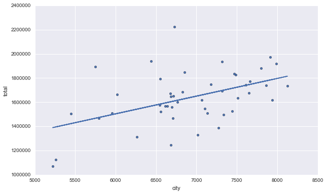
This is a medium correlation – not great, but not bad. I don’t have anything else to use, so let’s go with it. Our new adjusted revenue (adj_revenue) will not be in dollars. It’s a ratio of the amount taken in city-wide parking meters to the amount taken in by city workers.
meter_records['adj_revenue'] = meter_records['total'] / meter_records['city']
meter_records.head()| month | total | city | brinks | adj_revenue | |
|---|---|---|---|---|---|
| 0 | 1 | 2224277 | 6729 | 0 | 330.550899 |
| 1 | 2 | 1892672 | 5751 | 0 | 329.103113 |
| 2 | 3 | 1468074 | 6711 | 0 | 218.756370 |
| 3 | 4 | 1618966 | 7069 | 0 | 229.023341 |
| 4 | 5 | 1509195 | 7134 | 0 | 211.549622 |
Now let’s see the mean adjusted revenue for months when Brink’s was active (1) and not active (0).
meter_records.pivot_table(columns=['brinks'], values=['adj_revenue'])| brinks | 0 | 1 |
|---|---|---|
| adj_revenue | 247.104317 | 229.583858 |
The p-value
There’s definitely a difference, but is it random chance or is this actually significant? In order to find out, we want the p-value.
What is a p-value?
For a test of statistical significance, we start with the null hypothesis. It’s generally the opposite of what we’re testing for – the skeptic’s view. In this case, the null hypothesis is that there’s no relation between whether Brink’s was operating the meters and the amount of revenue brought in.
Once you have that, you compare your observed result – in this case the difference in mean adjusted revenue for months when Brink’s was active and when it was inactive – to some statistical model to see how extreme your result is. The p-value can be defined as “given your observed result, what’s the likelihood the null hypothesis is true?”
It has been generally accepted for years that a p-value of < 0.05 is statisically significant – we assume the null hypothesis is not true given a p-value that low. More recently, the idea of a bright line separating significant and non-significant p-values has been debated. While you should be careful with making the assumption that p < 0.05 means you’re in the clear, let’s go with it for this analysis.
Note that we never see the chance that our alternative hypothesis – the thing we’re testing for – is true. We are accepting or rejecting the null hypothesis.
Shuffling labels
There are complex formula-based ways to calculate the p-value. I don’t know them. I have a computer, though, so I can use another way. We can shuffle the labels – in this case, shuffle the “brinks” value to different months – many times and record our results. Shuffling them assume they don’t matter – our null hypothesis. If we do this many times, we can get a distribution of results and then see where our observed result falls on that. I’m going to do this with Pandas, but there’s other ways.
# Get our observed value.
def mean_revenue_diff(df):
    revenues = df.pivot_table(columns=['brinks'], values=['adj_revenue'])
    return (revenues[0] - revenues[1])['adj_revenue']

observed_mean_diff = mean_revenue_diff(meter_records)
observed_mean_diff 17.520458731191894# Copy the table so we can mess with it.
mr2 = meter_records.copy()
mr2.head()| month | total | city | brinks | adj_revenue | |
|---|---|---|---|---|---|
| 0 | 1 | 2224277 | 6729 | 0 | 330.550899 |
| 1 | 2 | 1892672 | 5751 | 0 | 329.103113 |
| 2 | 3 | 1468074 | 6711 | 0 | 218.756370 |
| 3 | 4 | 1618966 | 7069 | 0 | 229.023341 |
| 4 | 5 | 1509195 | 7134 | 0 | 211.549622 |
Shuffle the Brink’s column
Again, we shuffle this column in the assumption that our null hypothesis is true – Brink’s didn’t steal any money – and so it shouldn’t matter which month has which label.
# Assign a randomized series based on the brinks column to the brinks column.
mr2.brinks = np.random.permutation(mr2.brinks)
mr2.pivot_table(columns=['brinks'], values=['adj_revenue'])

mean_revenue_diff(mr2) 9.5953470328721266Let’s do this 10,000 times to get a good sampling.
num_experiments = 10000
results = []
count = 0
for _ in range(num_experiments):
    mr2.brinks = np.random.permutation(mr2.brinks)
    mean_diff = mean_revenue_diff(mr2)
    results.append(mean_diff)
    if observed_mean_diff >= 0 and mean_diff >= observed_mean_diff:
        count += 1
    elif observed_mean_diff < 0 and mean_diff <= observed_mean_diff:
count += 1print("Observed difference of two means: %.2f" % observed_mean_diff)
print(count, "out of", num_experiments, "experiments had a difference of two means ", end="")
if observed_mean_diff < 0:
print("less than or equal to ", end="")
else:
print("greater than or equal to ", end="")
print("%.2f" % observed_mean_diff, ".")
print("The chance of getting a difference of two means ", end="")
if observed_mean_diff < 0:
print("less than or equal to ", end="")
else:
print("greater than or equal to ", end="")
print("%.2f" % observed_mean_diff, "is", (count / float(num_experiments)), ".") Observed difference of two means: 17.52
285 out of 10000 experiments had a difference of two means greater than or equal to 17.52 .
The chance of getting a difference of two means greater than or equal to 17.52 is 0.0285 .That’s our p-value! Let’s see it on a graph.
plt.figure(figsize=(10, 6))
sns.distplot(results, kde=False)
plt.vlines(observed_mean_diff, 0, 600, colors="g", linestyle="dashed")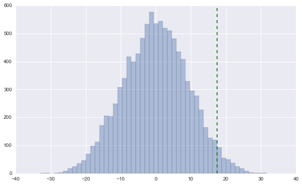
Confidence intervals
We’d like to know the amount of money Brink’s owes the city, but there’s not a good way to say exactly what that is.
Even though our results were statistically significant, they might not even be important. What if Brink’s employees stole $100/month? To NYC, the costs of taking the case to trial would dwarf that. Confidence intervals show us importance. A confidence interval is simply the range of likely results. In general, this is the middle 90% of possible values.
How do we get “possible values?” We can use a technique called “bootstrapping”. We create samples of the data the same size as the original, taking observations randomly and with replacement. This means that we might pick the same observation more than once – which is what we want. We do this 10,000 times, taking the difference of means each time.
# Notice the repetitions below -- this is because of replacement.
meter_records.sample(n=10, replace=True)| month | total | city | brinks | adj_revenue | |
|---|---|---|---|---|---|
| 28 | 30 | 1846508 | 6855 | 1 | 269.366594 |
| 19 | 21 | 1565671 | 6613 | 1 | 236.756540 |
| 7 | 8 | 1520443 | 6558 | 0 | 231.845532 |
| 37 | 39 | 1881303 | 7803 | 0 | 241.099962 |
| 15 | 17 | 1385822 | 7271 | 1 | 190.595792 |
| 44 | 46 | 1648605 | 6685 | 0 | 246.612565 |
| 41 | 43 | 1664116 | 6020 | 0 | 276.431229 |
| 45 | 47 | 1837134 | 7470 | 0 | 245.934940 |
| 41 | 43 | 1664116 | 6020 | 0 | 276.431229 |
| 11 | 13 | 1330143 | 7016 | 1 | 189.587087 |
conf_interval = 0.9
num_experiments = 10000
results = []
for _ in range(num_experiments):
    df = meter_records.sample(frac=1, replace=True)
    mean_diff = mean_revenue_diff(df)
    results.append(mean_diff)

results.sort()
tails = (1 - conf_interval) / 2
lower_bound = int(math.ceil(num_experiments * tails))
upper_bound = int(math.floor(num_experiments * (1 - tails)))

print("Observed difference between the means: %.2f" % observed_mean_diff)
print("We have %d%% confidence that the true difference between the means is between: %.2f and %.2f." % \
      (conf_interval * 100, results[lower_bound], results[upper_bound]))
Observed difference between the means: 17.52
We have 90% confidence that the true difference between the means is between: 2.63 and 32.78.plt.figure(figsize=(10, 6))
plt.axvspan(results[lower_bound], results[upper_bound], facecolor='g', alpha=0.2)
sns.distplot(results, kde=False)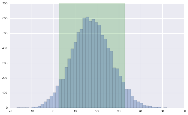
This doesn’t get us an amount of dollars, though. How could we do that?
I chose to get the mean amount of dollars the city workers brought in each month while Brink’s was active and multiply the adjusted revenue by that. This is the part of my analysis I feel most shaky about.
# Do amount of dollars calculations here.
meter_records[meter_records.brinks == 1].city.mean() 6933.75print(results[lower_bound] * 6933.75)
print(results[upper_bound] * 6933.75) 18225.8255225
227268.959718We have $20,525-230,372 per month. Let’s find out how many months Brinks was active to find out our totals.
num_months = len(meter_records[meter_records.brinks == 1])
num_months 24print(results[lower_bound] * 6933.75 * num_months)
print(results[upper_bound] * 6933.75 * num_months) 437419.81254
5454455.03323In total, it looks like Brink’s owes the city somewhere between $0.5 million and $5.5 million. That’s a large range – we didn’t have a lot of data, which often results in a large range – but it’s a good starting place, and shows that it’s definitely worth the city taking Brink’s to court. I looked up the actual judgment, and it appears NYC was awarded $1 million in compensatory damages and $1.5 million in punitive damages, which fits my results pretty well.